Mean Computation via Online Algorithms
Online learning theory has become one of my favorite subjects during my masters. Online learning happens via online algorithms which calculate or estimate some value from a continuous stream of incoming data. There are various different algorithms and there is a wide variation of influencing factors which can make the learning task difficult. In this blog post I want to look at computing the mean via online algorithms and how you can think about the behavior of some of these algorithms, and why that would be wanted or not.
The Regular Mean
The simplest computation you would need to make in any data related course is probably calculating the mean of a data set. And, despite this being such a simple thing to do, it is a very powerful and frequently used tool. So the first thing we will look at is how you calculate the regular mean using an online method. First, assume we have a data set \(x_1,\ldots,x_n\). Normally we express the mean of this data set as
\[\mu_n = \frac{1}{n} \sum_{i=1}^n x_i.\]For online learning however, we want this in the form of updates; describing how we need to adapt to new input rather than computing the thing in one go. We do this by rewriting the above formula to give this:
\[\begin{split}\mu_{n+1} &= \frac{1}{n+1} \sum_{i=1}^{n+1} x_i\\ &= \frac{n}{n+1} \left( \frac{1}{n} \sum_{i=1}^n x_i \right)+ \frac{1}{n+1} x_{n+1}\\ &= \frac{n}{n+1} \mu_n + \frac{1}{n+1} x_{n+1}.\end{split}\]Thus if we know the old mean \(\mu_n\) we can compute the new mean \(\mu_{n+1}\) without looking up old data points. To see this in action I’ve written a script in python which shows how this works, see this repo if you want to run it yourself. As a basic setup will feed a list of zeros and ones to the algorithm and it will calculate the ratio \(p\) between ones and zeros using this update rule.
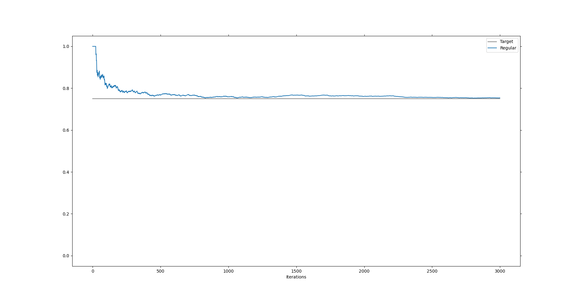
As we can see it converges nicely to the intended target. This is because even with randomness involved the mean converges quickly.
However, suppose we have the situation where our intended target switches for some reason. To give you a specific example, suppose we are the managers of a supermarket and we’ve been keeping track of the average amount of outgoing booze to ensure that we always have enough in stock. However, in 2019 the pandemic starts and now everyone is suddenly at home. There is a sudden change in booze supply. No longer do we supply the partying masses, but instead we supply the occasional drink on the couch. What happens to our algorithm if we keep it as is?
To see what happens let’s consider the case where we switch from target part way through the computation.
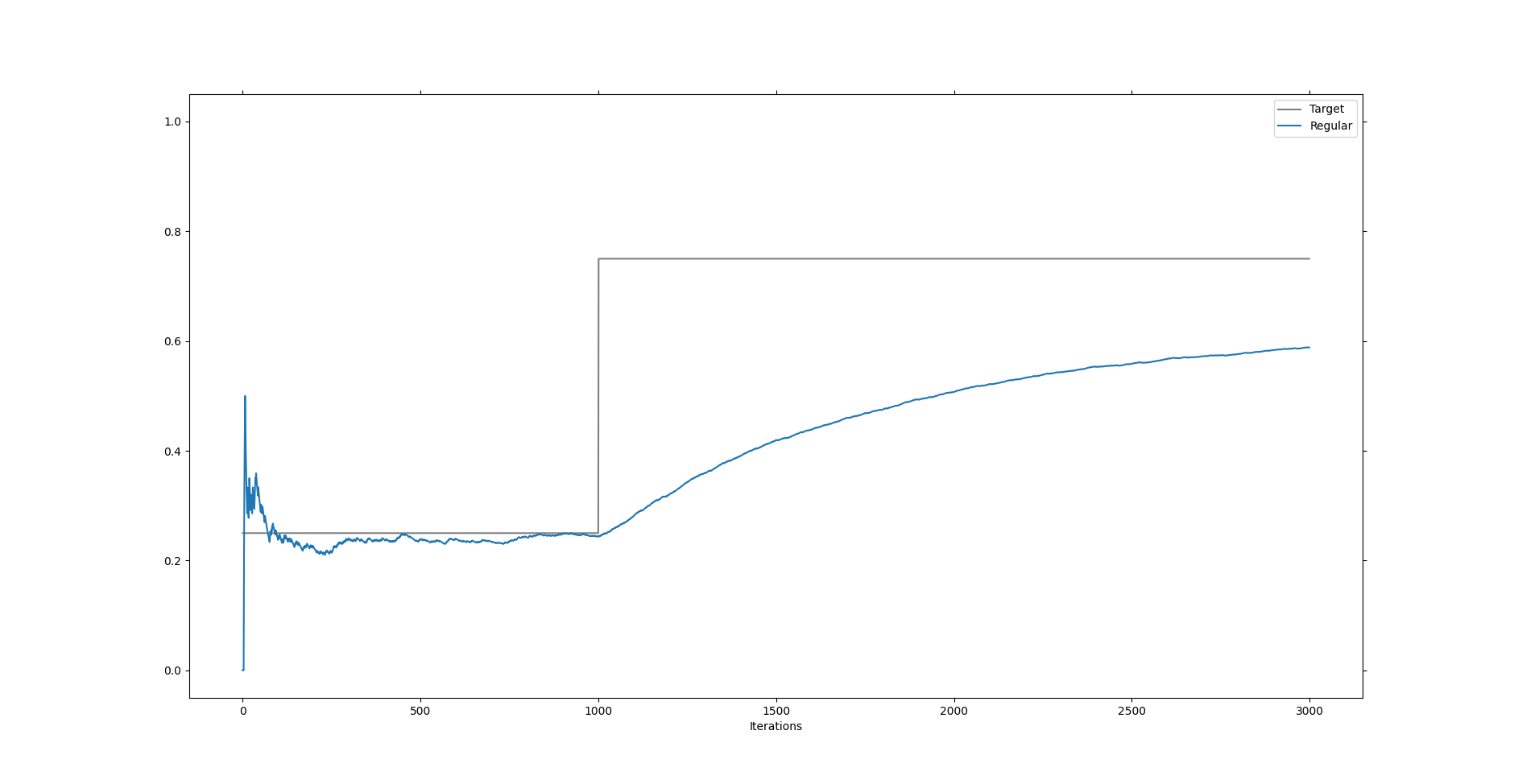
As we can see it takes the mean a long time before it is even half way to the new target. So if our supermarket managers started collecting data in 2015, then it will be a couple of years before they start getting good information again. And, who knows what else might happen in a couple of years. If the pandemic is over people might just starting going on a year long booze fest; another adjustment which we would need to wait on. This will not do.
The Exponential Mean
Of course, very clever people were dealing with this problem long before I did in this blog post. Well, they were dealing with the mathematics behind this, perhaps not with the booze logistics during a pandemic, though it wouldn’t be the first time that booze influenced mathematics, check out the history of Student’s t-test.
Leaving the booze behind and going back to our problem, there is a very simple thing you can do to get an algorithm which adjusts well to change. We change the update terms from \(n/(n+1)\) and \(1/(n+1)\) to some value \(a\) and \(1-a\) such that
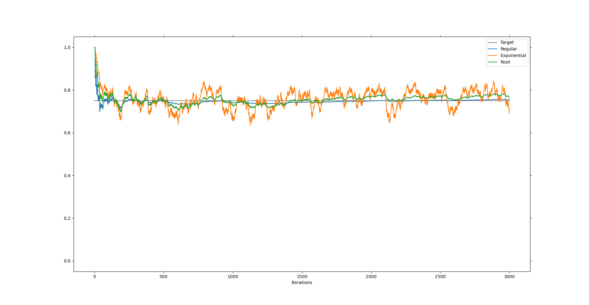
\[\mu_{n+1} = (1-a) \mu_n + a x_{n+1}.\]This creates an exponential mean, so called because older terms in the mean are repeatedly multiplied with \((1-a)\). Running this update rule in the unchanging and changing situations we get the following two plots.
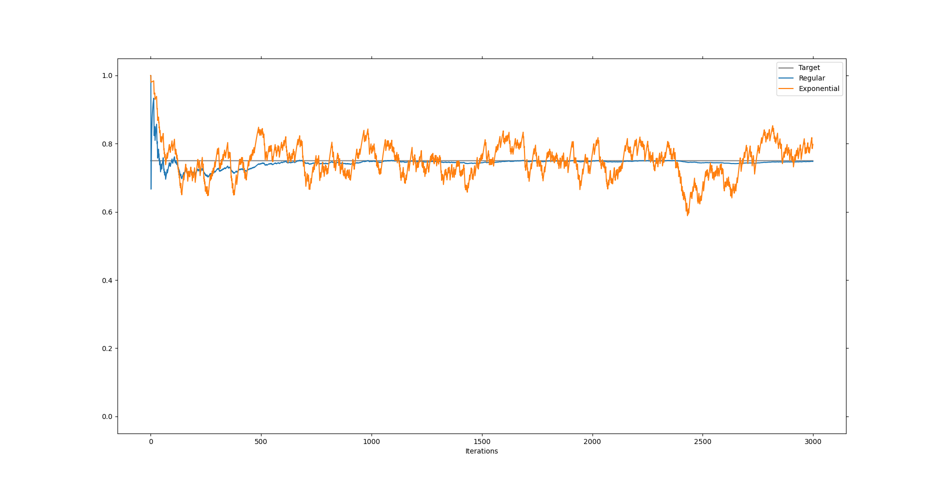
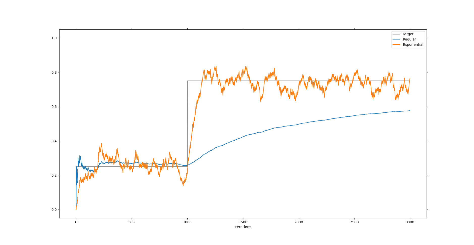
We can think \(a\) and \((1-a)\) as measures of trust. In essence we believe that \(x_{n+1}\) always holds the same amount of information compared to \(\mu_n\). In the computation for the regular mean we believe that \(x_{n+1}\) holds only \(1/(n+1)\) amount of information. This would be precisely an even spread among all received data points. But in calculating the exponential mean we want to quickly adapt to change and therefore we keep our belief to a steady amount, simply because we want to be as quickly as possible near the new value. You can see in the graphic that it is much better suited to finding the new value shortly after the change happened, but that it also never truly converges on the updated value.
This means that if our supermarket managers use this algorithm, they will sometimes be purchasing too much or too little booze, but also have a much easier time transitioning into the new situation. This is great around moments of change, but before and after this might not be all that it could be.
The Fancy Mean
Pandemics happen, but they don’t occur that often and we would not want to just throw away old but useful information. Alright, I might be stretching the example here, but what I am about to tell has a real use case. Suppose we know that there will be just one or two pandemics. We don’t know when they will happen but we do know that after those pandemics life will be eternal bliss with booze for everyone that wants it and no booze for people that don’t want it. How can our supermarket managers best deal with this situation? They want to do alright during the few pandemics and have an accurate reading after. Well, they adjust the belief to decrease slower than \(1/(n+1)\) but not so slow to stagnate on a non-zero value. For example, they could try the update rule
\[\mu_{n+1} = \left( 1- \sqrt{\frac{1}{n+1}} \right) \mu_n + \sqrt{\frac{1}{n+1}} x_{n+1}.\]This update rule puts more emphasis on the \(x_{n+1}\) terms than the regular mean because \(\sqrt{1/(n+1)}\) is always bigger than \(1/(n+1)\). Simultaneously, it does not put so much emphasis on this term to always believe it. Gradually, belief in the \(x_{n+1}\) term fades as \(n\) becomes bigger.
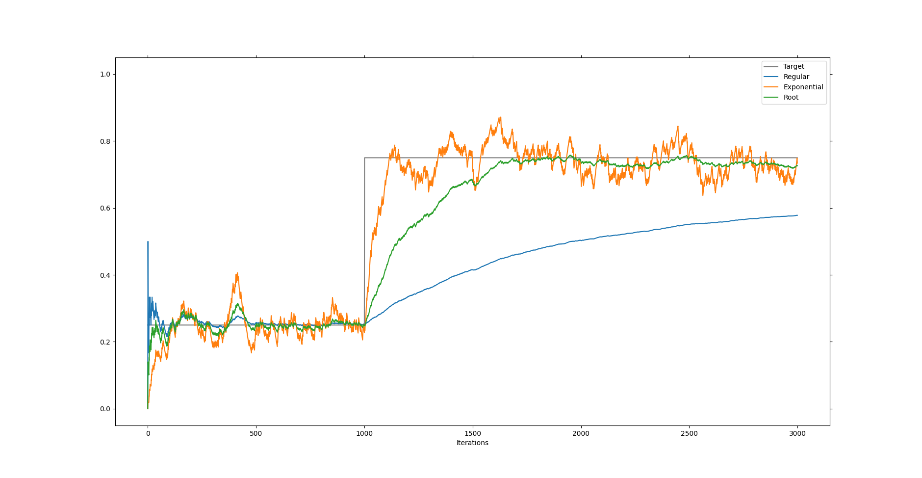
If we look at the behavior of this mean calculation we see that it does converge to the desired value and indeed it does update faster to the new value when the change occurs. However, it does so slower than the exponential mean. Of course, this is what is supposed to happen. The regular mean treats all moments in the past and future equally and thus has trouble adjusting to change. Contrary, the exponential mean doesn’t trust moments in the past and only those of the present and thus it keeps changing with new trends. The new update rule finds a sweet spot in between the two. It starts distrusting data points that are far away, but it doesn’t trust moments of the present as much if it has already experienced a lot. Thus it is still sensitive to the randomness but also gets more confident as time goes on.
By no means (pun intended) are any of these methods universally best. It depends all on the use case of the mean and the situation it finds itself in. There are also loads more variation of the update rule which will all behave differently. What is important though is that you now have an intuition in how these update rules work. You can use a bit of analysis and probability theory to make these examples rigid if you want, and that is a great exercise and helps sharpen your mathematical mind, but I think with a little bit of playing around that for practical cases you now have enough tools to recognize and analyze various online mean calculating algorithms.
Stay healthy and I’ll see you in the next post.